Bimodal GEV (generalized extreme value) distribution

Functions to compute the density, distribution function, quantile function, and to generate random variates for the BGEV (bimodal generalized extreme value)

Usage

dbgev(x, mu = 1, sigma = 1, xi = 0.3, delta = 2)

pbgev(q, mu = 1, sigma = 1, xi = 0.3, delta = 2)

qbgev(p, mu = 1, sigma = 1, xi = 0.3, delta = 2)

rbgev(n, mu = 1, sigma = 1, xi = 0.3, delta = 2)

Arguments

x

Numeric vector of values for calculating density.

mu

location parameter

sigma

scale parameter (sigma > 0)

xi

shape parameter in R

delta

shape parameter (delta > -1)

q

Numeric vector of quantiles.

p

Numeric vector of probabilities.

n

Number of observations for random generation.

Value

dbgev

density values

pbgev

distribution function values

qbgev

quantile function values

rbgev

random variates

Details

This distribution was proposed by Cira EG Otiniano, Bianca S Paiva, Roberto Vila and Marcelo Bourguignon (2021)

Note

BGEV distribution is equivalent to the GEV distribution when delta = 0. When comparing BGEV with GEV from package EnvStats, the shape parameter of GEV is changed to -xi due to reparametrization

References

Otiniano, Cira E. G., et al. (2023). A bimodal model for extremes data. Environmental and Ecological Statistics, 1–28. doi:10.1007/s10651-023-00566-7

Author

Thiago do Rego Sousa and Yasmin Lirio

Examples

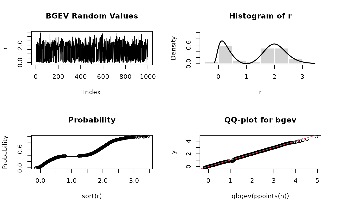
par(mfrow = c(2, 2))
set.seed(1000)
r <- rbgev(n = 1000)
plot(r, type = "l", main = "BGEV Random Values")

hist(r, probability = TRUE, border = "white", ylim = c(0,1))
x <- seq(min(r), max(r), length = 201)
lines(x, dbgev(x), lwd = 2)

plot(sort(r), (1:1000)/1000, main = "Probability", ylab = "Probability")
lines(x, pbgev(x), lwd = 2)

round(qbgev(pbgev(q = seq(0, 3, by = 0.1)), 6),2)
#>  [1] 5.0 5.1 5.2 5.3 5.4 5.5 5.6 5.7 5.8 5.9 6.0 6.1 6.2 6.3 6.4 6.5 6.6 6.7 6.8
#> [20] 6.9 7.0 7.1 7.2 7.3 7.4 7.5 7.6 7.7 7.8 7.9 8.0

n <- 10000
y <- rbgev(n)
qqplot(qbgev(ppoints(n)), y,
      main = "QQ-plot for bgev")
qqline(y, distribution = function(p) qbgev(p),
      probs = c(0.1, 0.6), col = 2)